Meteorology 101: How To Plot Wind Map
Well, Hello Friends!
This will be the second post explaining about meteorology. For those of you who missed the first post, you can check this link. In that post i explained about Meteorology 101: How to Download and Plot Meteorological Data from ERA5, which is this post will related and it seems like continuation from my first topic. So, you better check the first-post first!
Do you still remember what variables we have? Yes, one of them is 10m u-v component of wind. But, why are there two kinds of wind variables; u and v? What is the meaning of that?
Wind velocity is a three-dimensional vector quantity with small-scale random fluctuations in space and time superimposed upon a larger-scale organized flow. The three-dimensions are constructed on zonal, meridional, and vertical directions. It is considered in this form in relation to, for example, airborne pollution and the landing of aircraft [1]. The terms of zonal means “along a latitudinal circle” or in the “west–east” direction, meanwhile meridional means “along a longitudinal circle” or in the “north-south” direction. When zonal and meridional move horizontally, the vertical direction gives up and down direction (vertical motion).
But, in this topic we gonna talk about zonal-meridional direction (horizontal wind), which is denoted by “u-v” component of wind.
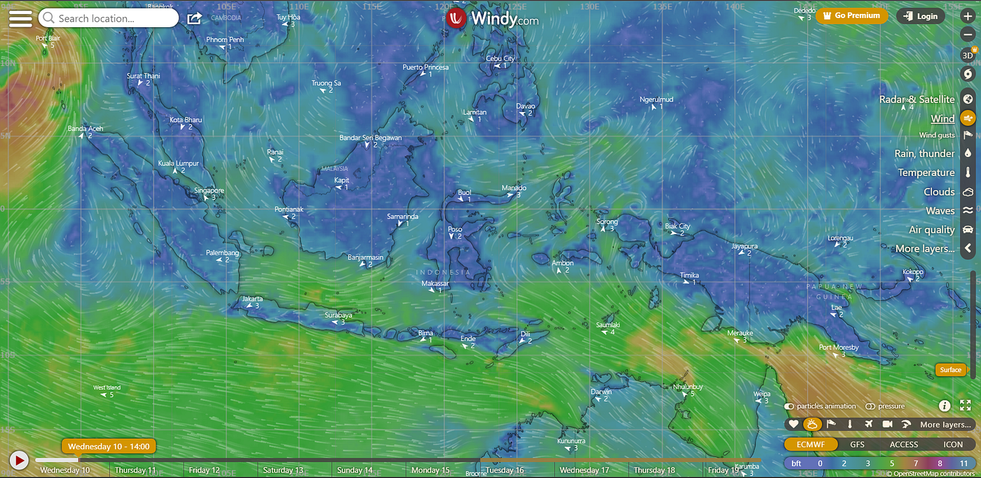
Air flow in the atmosphere has both a speed and direction. This is represented mathematically by a vector. Maps that show winds will also sometimes display them as vectors as shown in figure 1. The wind data from the numerical models and the objective analysis systems is always reported as the magnitude of the component vectors u and v like the data we have [2].
So, how do we calculate those the components to get the magnitude (wind speed) and directions?
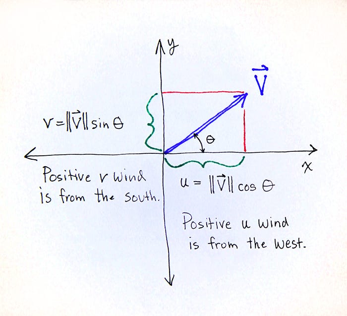
Given V (blue arrow) is the wind speed blowing from southwest, where positive v-wind is from the south and positive u-wind is from the west. To get know the magnitude or wind speed we can simply use Pythagorean Theorem; where V (blue arrow) is square root from the sum of u-v square. Then, to get the directions turn again to trigonometry. We have x and y (u and v), and we want an angle. This will require the inverse trig function of tan — eg, arctan(v/u) (for more explanation you can check here).
PLOT THE DATA
Then, how to plot the data?
Let’s open our jupyter notebook!
This is the library you have to declared.
import matplotlib.pyplot as plt
import pandas as pd
import numpy as np
import xarray as xr
from mpl_toolkits.basemap import Basemap
Next, open the ERA5 data.
data = xr.open_dataset('ERA5.nc')Define latitude and longitude coordinates as ‘lat’ and ‘lon’.
lat = data.latitude
lon = data.longitude
Define the u-v component of wind as ‘wind_u’ and ‘wind_v’.
wind_u = data.u10
wind_v = data.v10
At this point, you can choose the specific time you want to plot, either at certain hour or on average hour. For this tutorial, I’ll choose the time later during the visualization.
Then, based on explanation above, to get the magnitude or wind speed we can calculate the square root from the sum of u-v square which in this case is ‘wind_u’ and ‘wind_v’.
WS = np.sqrt(wind_u**2 + wind_v**2)Next, let’s load the map through the Basemap. The setting for the Basemap are still the same as before.
m = Basemap(projection='cyl', llcrnrlon=90, llcrnrlat=-15, urcrnrlon=150, urcrnrlat=15, resolution='i')
m.drawcoastlines(1)
m.drawcountries()

parallels = np.arange(-15,15+0.25,5)
m.drawparallels(parallels, labels=[1,0,0,0], linewidth=0.5)
meridians = np.arange(90,150+0.25,10)
m.drawmeridians(meridians, labels=[0,0,0,1], linewidth=0.5)
And here the visualization! For the time, i choose time = 5 or at 5 UTC as an example.
cf = plt.contourf(lon,lat,WS[5,:,:], cmap='jet')

cb = plt.colorbar(cf, fraction=0.0235, pad=0.03 )
cb.set_label('m/s',  fontsize=15)

plt.show()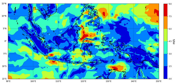
We can see from the figure 3 the distribution of wind speed over Indonesia at 05 UTC. The wind speed is in m/s scale. But, what about the direction of the wind speed?
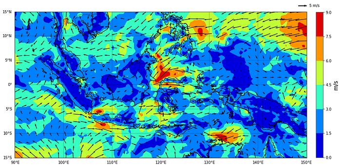
Well, to show the direction of wind speed we will use matplotlib feature; quiver plot. So what is quiver plot? quiver plot is basically a type of 2D plot which shows velocity vectors as arrows with components (u, v) at the points (x, y). You can read the documentation about quiver here.
So, how to use the quiver plot?
cf = plt.contourf(lon,lat,WS[5,:,:], cmap='jet')
Q = plt.quiver(lon[::6],lat[::6],wind_u[5,::6,::6],wind_v[5,::6,::6], scale_units='xy', scale=3, width=0.0015)

qk = plt.quiverkey(Q,
              1, 1.04,
               5,str(5)+' m/s',
               labelpos='E',
               coordinates='axes'
               )

cb = plt.colorbar(cf, fraction=0.0235, pad=0.03 )
cb.set_label('m/s',  fontsize=15)

plt.show()
Since the call signature of quiver is “quiver([X, Y], U, V, [C], **kwargs)”, which is X, Y is the arrow locations and U, V is the arrow of directions, we will define X, Y as ‘lon’ and ‘lat’ and U, V as ‘wind_u’ and ‘wind_v’, and C is optionally sets the color.
After we define and call the quiver plot, the visualization of wind map will be like this.
If you feel that the arrows is not tight enough, you can modify density of the arrows by setting the input of density. The density that i mean is [::6], which means it skips the arrow data value by 6. You can write code like this for efficiency.
skip = 6
quiver(lon[::skip],lat[::skip],wind_u[5,::skip,::skip],wind_v[5,::skip,::skip])
Lastly, quiverkey aims to provide settings regarding the quiver legend. I put it on the top-right and pointed to the east. The length of the arrow define the wind speed, which is it define 5 m/s. You can read the documentation about quiverkey here.
